GEMC Analyzer
analyzer is a small Python package for reading GEMC output files and plotting
variables by name. It currently focuses on CSV and ROOT output from gstreamer,
with a reader structure that can be extended to other formats later.
Dependencies
The analyzer dependencies (pandas, numpy, matplotlib) are pre-installed in the GEMC Python
environment (python_env/) created during meson install. No separate installation is needed when
using the python3 or gemc-analyzer commands from that environment.
ROOT output support also requires uproot, which can be added to the environment if needed:
pip install uproot
ROOT prerequisites:
- GEMC must be built with ROOT support and the ROOT streamer plugin available.
- The run must use gstreamer format root.
- Reading ROOT files from Python does not require importing C++ ROOT; the analyzer uses
uproot.
The dependency-free SVG helper in pygemc.analyzer.svg_plot only uses the Python standard library. It is useful on minimal systems where pandas, numpy, and matplotlib are not installed.
GEMC Output Model
The CSV streamer writes two flattened files per worker thread:
<rootname>_t<thread>_true_info.csv
<rootname>_t<thread>_digitized.csv
For one thread and filename: b2, the files are typically:
b2_t0_true_info.csv
b2_t0_digitized.csv
CSV files are read with:
pd.read_csv(path, sep=",", skipinitialspace=True)
The CSV rows include event context columns such as:
evn, timestamp, thread_id, detector
The digitized B2 output includes columns like:
hitn, pid, tid, E, time, totEdep
The true-info output includes tracking columns like:
processName, avgTime, avgx, avgy, avgz, hitn, pid, tid, mtid, vx, vy, vz, mvx, mvy, mvz, totalEDeposited
When the matching digitized CSV is available, the analyzer also adds E to true-info tables by matching rows on event, detector, hit, PID, and track ID. In that case E is the track total energy, while totalEDeposited remains the deposited energy.
The vx, vy, and vz columns are the current track vertex coordinates. The mvx, mvy, and mvz columns are the mother-track vertex coordinates when the mother track was available to GEMC hit processing; otherwise they use the GEMC uninitialized numeric sentinel. The mtid column stores the mother track ID.
Original-Track Differences
Upcoming in the next release: the analyzer derives momentum and direction changes for true-information hits when
GEMC saves the original-track information.
Enable save_original_track in the YAML configuration:
save_original_track: true
The true-information CSV then contains the original track ID and particle ID, together with the original momentum components:
otid, opid, opx, opy, opz
The current momentum components are px, py, and pz. When all these columns are present, the analyzer adds three plottable quantities:
| Quantity | Definition | Unit |
|---|---|---|
| delta_p | current momentum magnitude minus original momentum magnitude | MeV |
| delta_theta | current polar angle minus original polar angle | radians |
| delta_phi | current azimuthal angle minus original azimuthal angle | radians |
These values are calculated only when pid equals opid. A matching particle ID indicates that the hit was likely produced by the original particle; rows with different IDs are excluded from the delta histograms. The delta_phi difference is wrapped to the interval [-pi, pi] so tracks crossing the azimuthal boundary produce a small angular difference instead of a value close to 2 pi.
List the derived quantities available in a true-information CSV:
gemc-analyzer b2_t0_true_info.csv --data true_info
Plot each difference:
gemc-analyzer b2_t0_true_info.csv delta_p --data true_info
gemc-analyzer b2_t0_true_info.csv delta_theta --data true_info
gemc-analyzer b2_t0_true_info.csv delta_phi --data true_info
Use --pid to select one particle species. The B2 configuration generates protons, so its valid original-track
delta rows have PDG particle ID 2212:
gemc-analyzer b2_t0_true_info.csv delta_p --data true_info --pid 2212
A PID with no eligible delta rows displays a concise No plot created message and exits normally. For example,
B2 electron hits have pid 11 but opid 2212, so their original-track deltas are intentionally undefined.
The same filter is available through the Python API and for y-vs-x plots:
from pygemc import plot_variable, read_output

output = read_output("b2_t0_true_info.csv")
plot_variable(output, "delta_p", data="true_info", pid=2212, show=True)
When the run uses generated particles, the CSV streamer also writes a per-thread generated_tracked file holding the generated particle kinematics:
b2_t0_generated_tracked.csv
It includes columns like:
evn, timestamp, thread_id, bank, name, pid, type, multiplicity, p, theta, phi, vx, vy, vz
The analyzer reads it into the generated_tracked stream, exposing p (momentum), theta, and phi for plotting. When the selected stream is empty or lacks one of these, plot_variable() falls back to generated_tracked automatically.
The ROOT streamer writes one ROOT file per worker thread. For one thread and filename: b2, the file is typically:
b2_t0.root
The file contains trees named:
event_header
run_header
true_info_<detector>
digitized_<detector>
ROOT detector trees store vector branches. The analyzer flattens each vector element into one DataFrame row.
Python API
Read one digitized CSV file:
from pygemc import read_output

output = read_output("b2_t0_digitized.csv")
df = output.get_frame("digitized")
print(df.columns)
Read a CSV root name when both files exist:
from pygemc import read_output

output = read_output("b2_t0", kind="csv")
print(output.summary())
List the numeric quantities available to plot for a stream. The columns are only known after the data is read, so this is discovered at runtime rather than from a fixed list:
from pygemc import available_variables, read_output

output = read_output("b2_t0_generated_tracked.csv")
print(available_variables(output, data="generated_tracked"))
# {'evn': 'evn', 'pid': 'pid', 'multiplicity': 'Multiplicity',
#  'p': 'Momentum (MeV)', 'theta': 'Theta (rad)', 'phi': 'Phi (rad)'}
Plot totEdep grouped by pid:
from pygemc import plot_variable, read_output

output = read_output("b2_t0_digitized.csv")
plot_variable(
    output,
    "totEdep",
    data="digitized",
    bins=30,
    xlim=(0.0, 0.1),
    show=True,
)
Read ROOT output:
from pygemc import read_output

output = read_output("b2_t0.root", kind="root")
df = output.get_frame("digitized", detector="flux")
Command-Line Usage
The gemc-analyzer command is installed into the GEMC Python environment and is available once
python_env/bin is on your PATH. It can also be invoked as python3 -m pygemc.analyzer.
Print a summary:
gemc-analyzer digitized.csv
Discovering Plottable Quantities
The quantities available to plot are the numeric columns of the file you load, so they are only known after
the data is read. They are not part of --help, which is the static argument list printed before any file is
opened.
To see them, run the analyzer without a variable. The summary is followed by a plottable <stream>: ... line
for each stream that is present:
gemc-analyzer digitized.csv
plottable digitized: E, evn, hitn, pid, tid, time, totEdep
plottable generated_tracked: evn, multiplicity, p, phi, pid, theta
Then plot a name from that list, for example the generated momentum:
gemc-analyzer b2_t0_generated_tracked.csv p
Plot a digitized variable with matplotlib:
gemc-analyzer digitized.csv totEdep --kind csv --xlim 0.0 0.1
Save a plot instead of showing it:
gemc-analyzer digitized.csv totEdep --kind csv --save b2_totEdep.png
Plot ROOT output with matplotlib:
gemc-analyzer b2_t0.root totEdep --kind root --detector flux --save b2_totEdep.png
Plot a true-info track vertex coordinate:
gemc-analyzer true_info.csv vx --kind csv --data true_info --save b2_vertex_x.png
Plot the generated particle quantities. A .csv file is auto-detected, and the generated p, theta, and
phi resolve from the generated_tracked stream automatically, so neither --kind csv nor --data
generated_tracked is needed:
gemc-analyzer b2_t0_generated_tracked.csv p --save b2_gen_p.png
gemc-analyzer b2_t0_generated_tracked.csv theta --save b2_gen_theta.png
gemc-analyzer b2_t0_generated_tracked.csv phi --save b2_gen_phi.png
Analyzer Plot Examples
The examples below were produced from 1000-event GEMC CSV runs. The -n=1000
command-line option overrides the event count for the run without modifying the
YAML file.
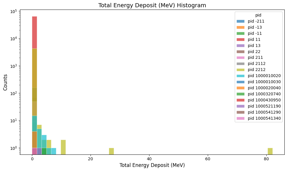
Plot the total energy deposited in the B2 digitized output:
gemc-analyzer digitized.csv totEdep --kind csv --bins 50
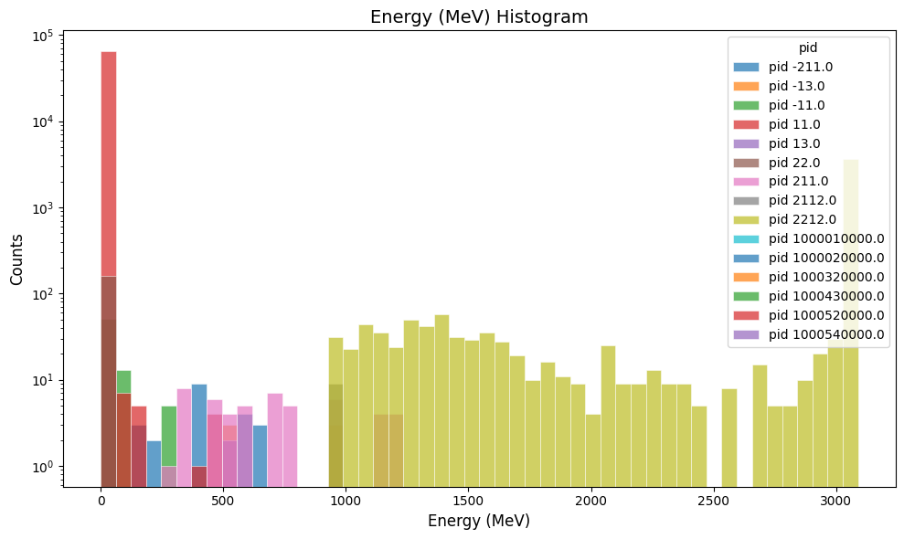
Plot the true-info track energy in the B2 output:
gemc-analyzer true_info.csv E --kind csv --data true_info --bins 50
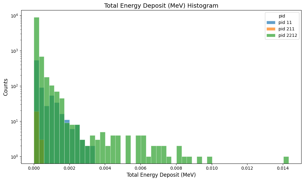
Plot the total energy deposited in the simple_flux digitized output:
gemc-analyzer digitized.csv totEdep --kind csv --bins 50
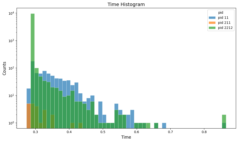
Plot the hit time in the simple_flux digitized output:
gemc-analyzer digitized.csv time --kind csv --bins 50
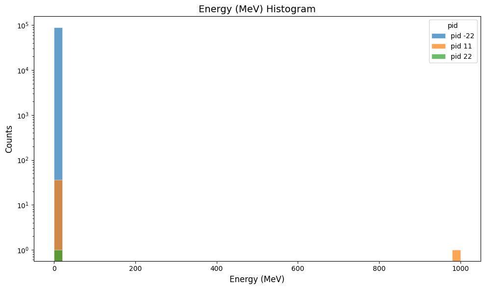
Plot the particle energy in the cherenkov digitized output:
gemc-analyzer digitized.csv E --kind csv --bins 50
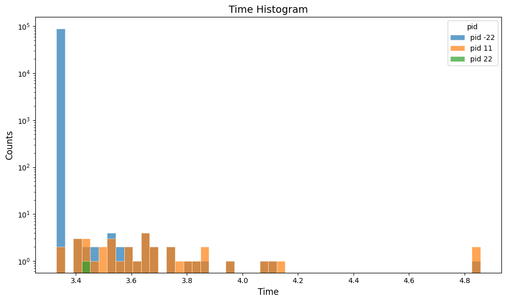
Plot the hit time in the cherenkov digitized output:
gemc-analyzer digitized.csv time --kind csv --bins 50
Jupyter Usage
The analyzer can also be used directly in notebook-style Python cells:
#%%
from pygemc import read_output, plot_variable

plot_variable(
    read_output("cherenkov_t0_digitized.csv"),
    "totEdep",
    data="digitized",
    bins=30,
    show=True,
)
Dependency-Free SVG Plot
If pandas, numpy, or matplotlib are unavailable, create an SVG histogram directly from the CSV file:
python3 -m pygemc.analyzer.svg_plot b2_t0_digitized.csv totEdep --out b2_totEdep.svg --bins 30
Add an x-axis range with:
python3 -m pygemc.analyzer.svg_plot b2_t0_digitized.csv totEdep --out b2_totEdep.svg --bins 30 --xlim 0.0 0.1
Run the B2 Example
Run these commands from the GEMC source directory.
Build the B2 geometry into a local SQLite database:
python3 examples/basic/b2/b2.py -f sqlite -sql gemc.db
Run GEMC with CSV output rooted at b2:
build/gemc examples/basic/b2/b2.yaml \
  '-gsystem=[{name: b2, factory: sqlite}]' \
  '-gstreamer=[{format: csv, filename: b2}]' \
  -sql=gemc.db \
  -n=1000
With one worker thread, this produces:
b2_t0_digitized.csv
b2_t0_true_info.csv
Inspect the digitized CSV header:
head -1 b2_t0_digitized.csv
Expected columns include:
evn, timestamp, thread_id, detector, hitn, pid, tid, E, time, totEdep
Create the totEdep plot with the main analyzer API:
gemc-analyzer digitized.csv totEdep --kind csv --save b2_totEdep.png
Or create the same style of histogram without third-party Python packages:
python3 -m pygemc.analyzer.svg_plot b2_t0_digitized.csv totEdep --out b2_totEdep.svg --bins 30
Run B2 With ROOT Output
To produce ROOT output instead of CSV, keep the same gemc.db and run:
build/gemc examples/basic/b2/b2.yaml \
  '-gsystem=[{name: b2, factory: sqlite}]' \
  '-gstreamer=[{format: root, filename: b2}]' \
  -sql=gemc.db \
  -n=1000
With one worker thread, this produces:
b2_t0.root
Read the ROOT file from Python if you want to inspect or manipulate the data before plotting:
from pygemc import plot_variable, read_output

output = read_output("b2_t0.root", kind="root")
print(output.summary())

df = output.get_frame("digitized", detector="flux")
print(df[["pid", "totEdep"]].head())

plot_variable(
    output,
    "totEdep",
    data="digitized",
    detector="flux",
    bins=30,
    show=True,
)
The Python inspection step is not required for plotting. To plot directly from the command line, use:
gemc-analyzer b2_t0.root totEdep --kind root --detector flux --save b2_root_totEdep.png
If matplotlib reports that its default cache directory is not writable, set a writable MPLCONFIGDIR:
MPLCONFIGDIR=. gemc-analyzer b2_t0.root totEdep --kind root --detector flux --save b2_root_totEdep.png
Extending Readers
New formats should return a GemcOutput object from analyzer.dataset.
Populate one or more of these maps:
GemcOutput(
    true_info={"name": true_info_dataframe},
    digitized={"name": digitized_dataframe},
    headers={"event_header": event_header_dataframe},
)
Then add the format selection to read_output() in analyzer/readers.py.