GUI Analyzer
The Analyzer plots numeric values produced by sensitive-detector plugins while GEMC is running. It discovers the plugin names and variables from the data itself, including dynamically loaded plugins; plugins do not need to declare a separate analysis schema.
The accumulator exists only in GUI mode. Batch runs do not create it and therefore do not pay its CPU or memory cost.
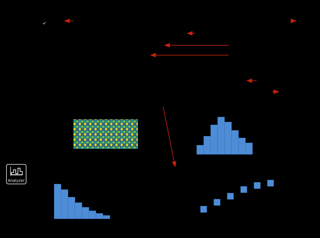
Discover and plot variables
The selectors are empty before the first run because the available data depends on the active geometry, plugins, and plugin implementation.
- Start GEMC with
-guiand click Run, or issue a Geant4beamOncommand. - Open Analyzer after the run completes.
- Select the Run and Plugin / detector.
- Select True information or Digitized. This one choice applies to both axes of a 2D plot.
- Choose 1D and an X variable, or choose 2D and both X and Y variables.
Each worker thread collects into its own shard. GEMC merges the shards under a mutex when the run finishes, so the displayed series includes samples from every worker without concurrent writes to a shared histogram. For a 2D plot, X and Y values are paired by the originating detector record rather than by merge order.
Changing the geometry clears the accumulated data. Run again to discover the variables exposed by the new configuration.
Plot controls
| Control | Effect |
|---|---|
| Accumulate | Preserve samples and append the results of later beamOn runs. |
| 1 plot / 4 plots | Switch between one chart and an equal-size 2×2 grid. |
| Position tabs | Configure Top Left, Top Right, Bottom Left, or Bottom Right. |
| 1D / 2D | Draw a histogram of X or a histogram of Y versus X. |
| 2D style | Draw the 2D bins as a heatmap or boxes. |
| Bins | Set the number of bins; in 2D the value applies to each axis. |
| Title | Override the automatic run, detector, source, and variable title. |
| X/Y minimum and maximum | Set each limit independently, or keep its own Auto checkbox selected. |
| Y scale / Z scale | Use a linear or logarithmic count scale; 2D plots apply it to Z. |
| Export PDF… | Save the chart configured by the current tab as a vector PDF. |
The four configuration panels live in tabs above the charts, leaving the 2×2 grid entirely available for the plots. All four grid cells have the same dimensions.
Prepare plots in YAML
Use ganalysis_plots and ganalysis_accumulate for the initial page state. Add one ganalysis entry per
plot position. This example prepares a 2D Simple Flux plot of avgy versus avgx:
ganalysis_plots: 1
ganalysis_accumulate: false

ganalysis:
  - position: top_left
    run: 1
    plugin: flux
    source: true
    dimension: 2d
    x: avgx
    y: avgy
    bins: 80
    x_min_auto: false
    x_max_auto: false
    y_min_auto: false
    y_max_auto: false
    x_min: -0.25
    x_max: 0.25
    y_min: -0.25
    y_max: 0.25
    title: Average Y Position vs Average X Position
    style: heatmap
    scale: linear
position accepts top_left, top_right, bottom_left, and bottom_right. source accepts true or
digitized; dimension accepts 1d or 2d; style accepts heatmap or boxes; and scale accepts
linear or logarithmic.
Configured variable names are non-editable and red until the first completed run validates them. A name that is absent from that run remains red and is labeled Not available. This lets one configuration describe a future runtime plugin without requiring GEMC to know its variables in advance.
Simple Flux example
The Simple Flux example records track information when particles cross its flux plane. The plot below uses 10,000 events, true information, 80 bins per axis, and independent avgx and avgy limits of -0.25 cm to 0.25 cm.
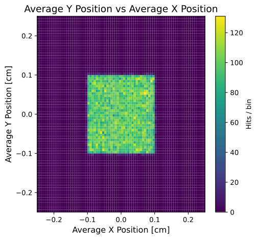
The plotted quantities are discovered after beamOn; they are not special-cased in the Analyzer.