Simple Flux Detector

This example uses the flux digitization to save true and digitized information in the output.

You can run this example in your browser:

Quickstart

Copy the example to your current directory. To create the geometry, run 10 events, and produce ROOT and CSV output files:

cp -r $GEMC_HOME/examples/basic/simple_flux .
cd simple_flux
./simple_flux.py
gemc simple_flux.yaml -n=10

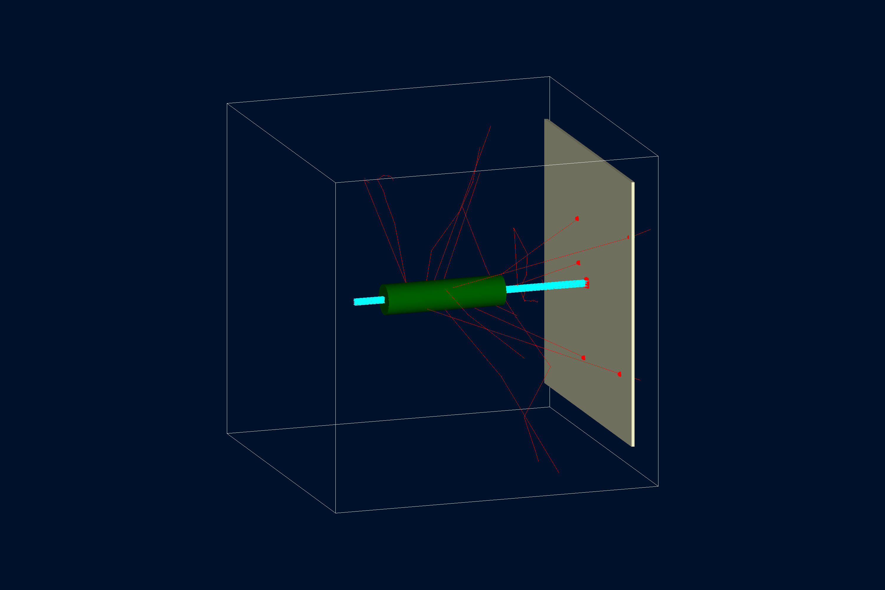
Geometry

The geometry, shown below, is defined in simple_flux.py.

The world (a box named root) contains:

target, a cylindrical liquid hydrogen target (G4_lH2)
FluxPlane, a box made of air (G4_AIR) and assigned the flux digitization

Interactive viewer:

Physics List

QBBC is used by default, selected in the YAML file with phys_list: QBBC.

phys_list

The physics list can be selected using the option
gemc -phys_list <value>
where <value> can be a combination of the Geant4 physics constructors separated by the + sign. For example
gemc -phys_list="FTFP_BERT + G4NeutronCrossSectionXS"
To see a list of the available Geant4 constructors:
gemc -showPhysics

Generator

The particle kinematics are defined in the YAML file:

gparticle:
  - name: proton
    p: 2000*MeV
    vz: -3*cm
    delta_vx: 0.1*cm
    delta_vy: 0.1*cm
    multiplicity: 10

See also the Internal Generator Documentation for more information.

Digitization

The FluxPlane sensitivity is specified with the flux digitization (one of the available GEMC prebuilt routines) in simple_flux.py, with identifier flux_plane = 1.

gvolume.digitization = "flux"
gvolume.set_identifier("flux_plane", 1)

In this case, the identifier contains one name: flux_plane.

See the Flux Documentation for more information.

In addition to the digitized variables, the true information is saved on the output stream.

True Information

The true information is processed by GEMC and, in some cases, averaged and weighted by the energy deposition. For variables like pid, tid, or processName, the data come from the first step in the hit.

The complete list of variables is:

the sensitive element identifier, assigned by the user. For example:

sector

layer

hitn: hit number

pid: particle ID

tid: track ID

avgTime: average time

avglx: average local x position

avgly: average local y position

avglz: average local z position

avgx: average global x position

avgy: average global y position

avgz: average global z position

totalEDeposited: total energy deposited

processName: process name creating the first step of this hit

Usage

Building the detector

Use the Python script simple_flux.py to build the detector. By default, the setup is stored in a SQLite file named gemc.db. Command-line options can define the database type, variations, and run number.

See also the Building Geometry for more information.

Running GEMC

The file simple_flux.yaml can be used to run the setup. Add -gui to run interactively:

gemc simple_flux.yaml -gui

Modify simple_flux.yaml as needed, in particular to add particles, control the number of threads, or change the output.

Running Events

Simple flux simulation: proton tracks traversing the flux detector volumes.

Output

The gstreamer option selects the output filenames and the format:

gstreamer:
  - format: csv
    filename: simple_flux

Because flux is a per-event digitization, GEMC will produce one output file per thread. For ROOT files, you can use hadd to merge the files.

See also the Output Documentation for more information.

Plotting with the GEMC Analyzer

Run GEMC with 10,000 events first. The default YAML file writes the analyzer CSV streams.

gemc simple_flux.yaml -n=10000

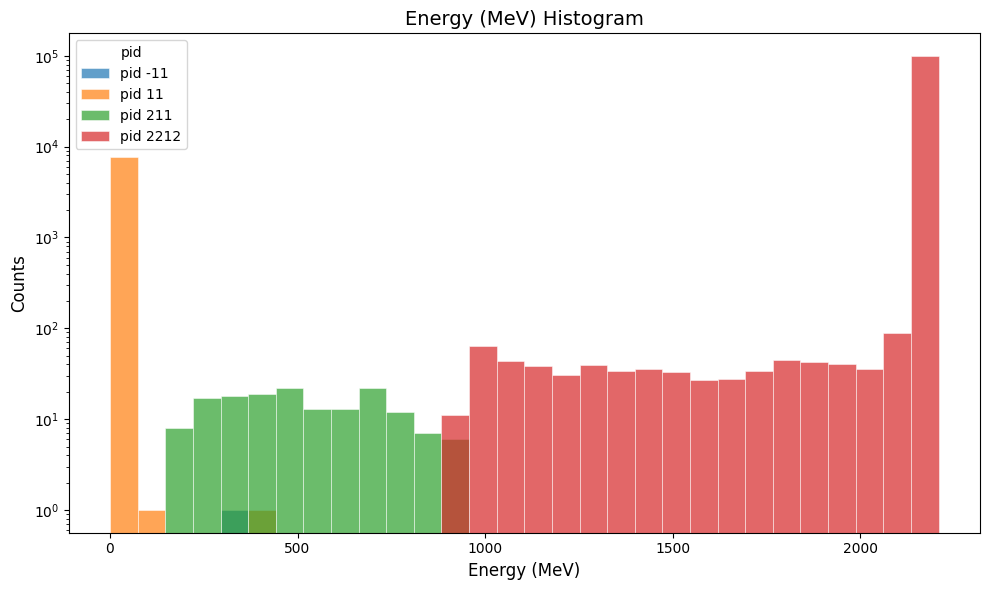
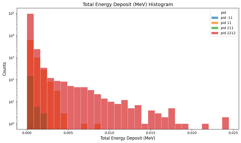
Plot the total energy deposited per hit:

gemc-analyzer simple_flux_t0_digitized.csv totEdep --kind csv

Simple Flux total energy deposited per hit

Plot the true particle track energy:

gemc-analyzer simple_flux_t0_true_info.csv E --kind csv --data true_info

Simple Flux true particle track energy