Example b1

This example reproduces the Geant4 basic example B1. It uses the dosimeter digitization to store the accumulated dose on a detector.

You can run this example in your browser:

Quickstart

Copy the example to your current directory. To create the geometry, run 10 events, and produce ROOT and CSV output files:

cp -r $GEMC_HOME/examples/basic/b1 .
cd b1
./b1.py
gemc b1.yaml -n=10

Geometry

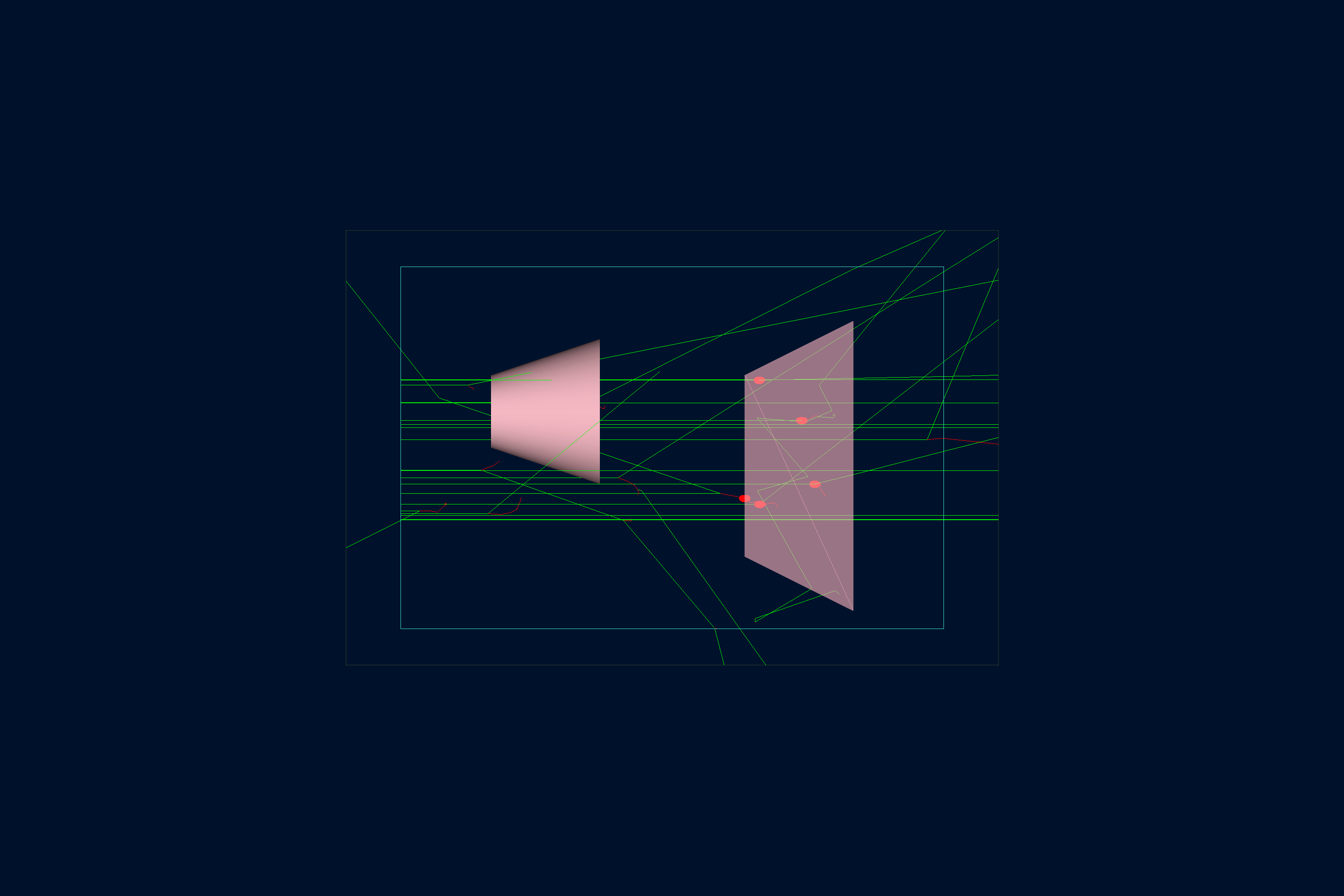
The geometry, shown below, is defined in b1.py.

The world (a box named root) contains:

Envelope, another box made of water.
Shape1 and Shape2, a polycone and a trapezoid, placed inside Envelope. These are made from tissue and bone materials, common for medical applications and thus pre-defined in the Geant4 Material Database:
- G4_A-150_TISSUE
- G4_BONE_COMPACT_ICRU

Interactive viewer:

Physics List

QBBC is used by default, selected in the YAML file with phys_list: QBBC.

phys_list

The physics list can be selected using the option
gemc -phys_list <value>
where <value> can be a combination of the Geant4 physics constructors separated by the + sign. For example
gemc -phys_list="FTFP_BERT + G4NeutronCrossSectionXS"
To see a list of the available Geant4 constructors:
gemc -showPhysics

Generator

The default kinematics is a 6 MeV gamma generated along the z-axis and randomly distributed in front of the envelope. This is defined in the YAML file:

gparticle:
  - name: gamma
    p: 6
    vz: -15
    delta_vx: 4
    delta_vy: 4
    multiplicity: 1

gparticle

The gparticle option allows to control the Geant4 particle gun. For the complete list of parameters that can be passed to it: gemc help gparticle.

Some of them:

name: Particle name (mandatory), for example “proton”.

multiplicity: How many copies of this particle will be generated in each event. notice that the copies are not identical if some additional parameters are specified, for example delta_p, delta_theta.

p: Particle momentum.

delta_p: Particle momentum range, centered on p.

theta: Particle polar angle.

delta_theta: Particle polar angle range, centered on theta. D

phi: Particle azimuthal angle.

For example, to define a particle gun with one electron along z plus 1 proton at theta=30,phi=90 degrees, use
Command line:
-garticle="[{name: e-, p: 5000}, {name: proton, p: 2000, theta: 30, phi: 90}]"
Yaml:
 particle:
  - name: e-
    p: 5000
    multiplicity: 5
  - name: proton
    p: 2000
    theta: 30
    phi: 90

Digitization

The Shape2 volume is associated to the dosimeter digitization (one of the available GEMC pre-built routines) in b1.py:

gvolume.digitization = 'dosimeter'
gvolume.set_identifier('mydosimeter', 1)

The dosimeter digitization will create and accumulate the variables etot and dose throughout events in a run.

\[\mathrm{dose} = \frac{\mathrm{etot}}{\mathrm{mass}}\]

where etot is the total energy deposited in each event and mass is the mass of Shape2.

Here, the custom string mydosimeter and number 1 identify the sensitive element.

The variables mydosimeter, etot and dose are saved in the output.

Usage

Building the detector

Use the Python script b1.py to build the detector. By default, the setup is stored in a SQLite file named gemc.db. Command-line options can define the database type, variations, and run number.

python API

Pass -h for additional command line options:

options:
  -h, --help            show this help message and exit
  -f, --factory FACTORY
						ascii, sqlite
  -v, --variation VARIATION
                        Set variation name
  -r, --run RUN         Set run number
  -sql, --dbhost DBHOST
                        SQLite filename or MYSQL host
  -pv, --pyvista        Show geometry using pyvista (needs pyvista)
  -pvb, --pvb, --pyvista-background
                        Use PyVista BackgroundPlotter (needs pyqt6 pyvistaqt)
  -pvw, --width WIDTH   Set plotter width
  -pvh, --height HEIGHT
						Set plotter height
  -pvx, --x X           Set plotter x position
  -pvy, --y Y           Set plotter y position
  -axes, --add_axes_at_zero

If you have pyvista (see also install pyvista), you can use the -pv and -pvb options to display the setup without having to run GEMC

Running GEMC

The file b1.yaml can be used to run the setup. Add -gui to run GEMC interactively:

gemc b1.yaml -gui

Modify b1.yaml or the command line as needed, in particular to add particles, control the number of threads, or change the output.

Output

The gstreamer option is used to select the output name and format. The YAML file writes simultaneous CSV and ROOT streams:

gstreamer:
  - format: csv
    filename: CO2
  - format: root
    filename: CO2

gstreamer

The gstreamer option allows select the name and format of the output. Run gemc help gstreamer to check its documentation:

-gstreamer=<sequence> ......: define a gstreamer output

• filename: name of output file. Default value: NODFLT
• format: format of output file. Default value: NODFLT
• type: type of output fileDefault value: event


Define output formats and filenames. 
It can be used to select <events> or <frame> streams.
The file extension is added automatically based on the format.

Supported formats:
	
  - jlabsro
  - root
  - ascii
  - csv
  - json


Output types:

  - event: write events
  - stream: write frame time snapshots

Example that defines two gstreamer outputs:

 -gstreamer="[{format: root, filename: out}, {format: csv, filename: out}]"


The produced files structure depends on the accumulation method used:

  - event-based digitization (like <flux>) will have one file per 
    thread, with "_t<thread#>" appended to the filename
  - run-based digitization (like <dosimeter>) will have one output file

Plotting with the GEMC Analyzer

Run GEMC with 1,000 events first. The default YAML file writes CO2_t0_digitized.csv.

gemc b1.yaml -n=1000

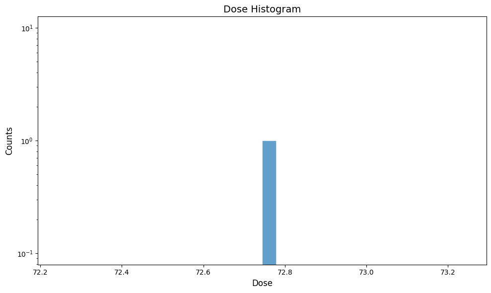
Plot the accumulated dose:

python3 -m analyzer CO2_t0_digitized.csv dose --kind csv

b1 dose plot

Plot the deposited energy:

python3 -m analyzer CO2_t0_digitized.csv etot --kind csv

b1 deposited energy plot