CAD Example
This example imports three STL organ meshes with the GEMC CAD factory and models a medical
brachytherapy treatment: an Iridium-192 high-dose-rate (HDR) source is placed inside the liver
and emits photons isotropically. Each organ is a flux sensitive detector, so the deposited energy
is recorded per organ; plot_dose.py converts it to absorbed dose and to the equivalent Ir-192
irradiation time.
Quickstart
Copy the example to your current directory. To upload the CAD definitions, run 200 events producing CSV output, and plot the dose in each organ:
cp -r $GEMC_HOME/examples/basic/cad .
cd cad
./cad.py
gemc cad.yaml -n=200
./plot_dose.py
Geometry
The geometry is defined declaratively in stls/cad__default.yaml and uploaded into gemc.db by
cad.py.
The CAD system named stls contains:
- heart_NIH3D, a blood-material heart mesh.
- respiratory_NIH3D, a translucent lung mesh made with G4_LUNG_ICRP.
- liver_NIH3D, a soft-tissue liver mesh.
Each entry in stls/cad__default.yaml sets the mesh file, material, color, scale, position, and
identifier. The system value must match both the gsystem name in cad.yaml and the directory
that contains the STL files. The three organs are centred on the y-axis (each centroid has
x = z = 0) and stacked along y, and the lung mesh — authored trachea-down — carries a 180° rotation
about z that turns it right-side up.
See also the CAD Imports Documentation for more information.
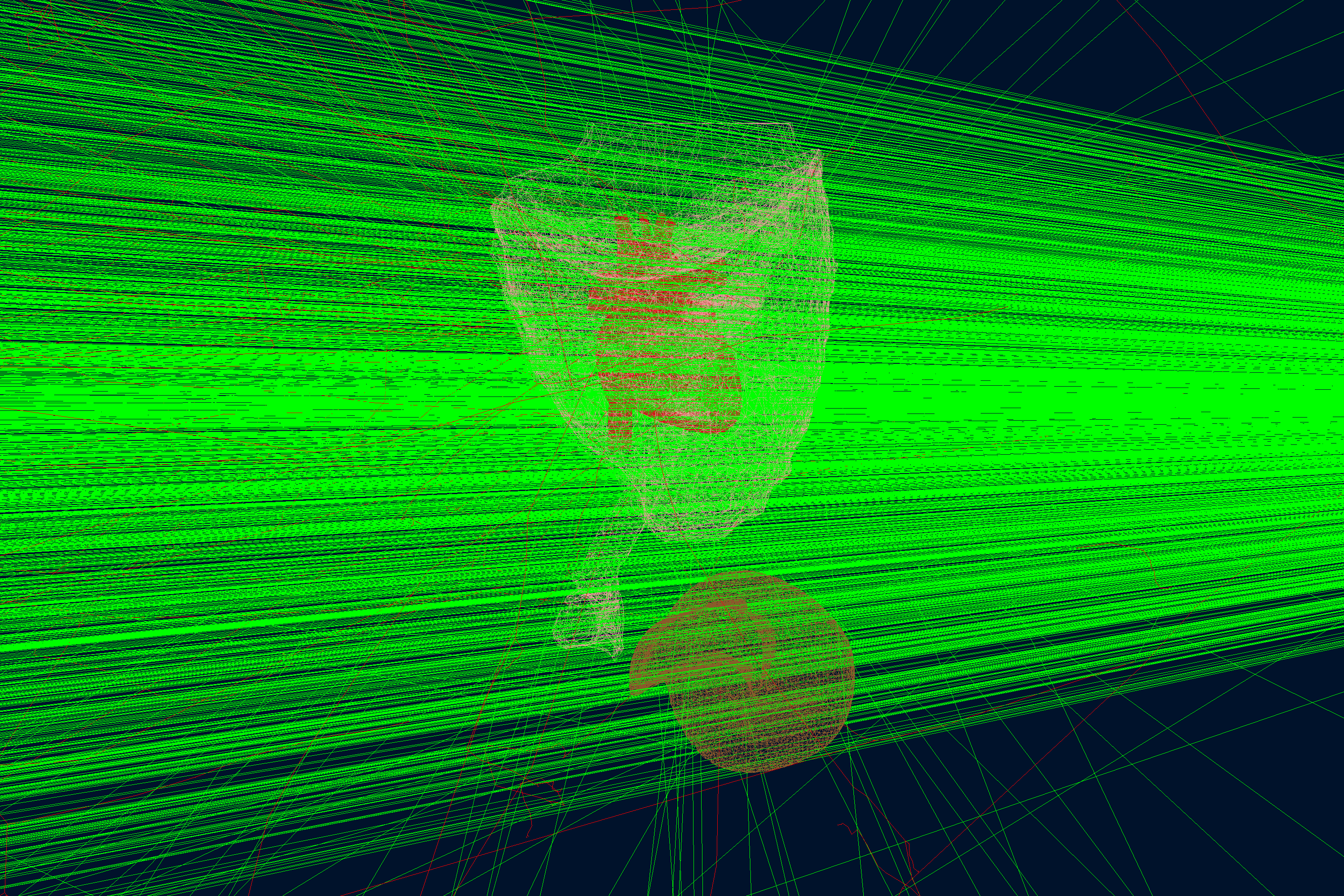
Interactive viewer:
Physics List
FTFP_BERT is used by default, selected in the YAML file with phys_list: FTFP_BERT.
phys_list
The physics list can be selected using the option
gemc -phys_list <value>where
<value>can be a combination of the Geant4 physics constructors separated by the+sign. For examplegemc -phys_list="FTFP_BERT + G4NeutronCrossSectionXS"To see a list of the available Geant4 constructors:
gemc -showPhysics
Generator
The particle kinematics are defined in the YAML file:
gparticle:
  - name: gamma
    p: 380*keV
    delta_p: 120*keV
    multiplicity: 300
    theta: 90*deg
    delta_theta: 90*deg
    randomThetaModel: cosine
    phi: 180*deg
    delta_phi: 180*deg
    vx: 0*mm
    vy: -140*mm
    vz: 0*mm
    delta_vx: 20*mm
    delta_vy: 20*mm
    delta_vz: 20*mm
    randomVertexModel: sphere
This models a clinical Iridium-192 HDR brachytherapy source loaded into the liver:
- Energy — Ir-192 emits a line spectrum (dominant lines 0.30–0.61 MeV). It is approximated here
by photons at the ~0.38 MeV mean photon energy, smeared with
delta_pto span the spectrum. - Position — the vertex is the liver centroid in world coordinates,
(0, -140, 0) mm, spread uniformly inside a ~35 mm sphere (randomVertexModel: sphereuses|delta_v|as the radius) to mimic the loaded dwell region. The organs are stacked along the y-axis (x = z = 0) with the heart at the origin, the liver just below it and the lungs above. - Direction — isotropic 4π emission:
cosinesampling of θ over 0–180° combined with a uniform φ over 0–360°.
See also the Internal Generator Documentation for more information.
Digitization
Each organ is configured as a flux sensitive detector in stls/cad__default.yaml:
defaults:
  digitization: flux

volumes:
  - name: heart_NIH3D
    identifier: "organ: 1"
The flux digitization is an event-mode detector: it writes one output row per hit, each row carrying the organ identifier and the deposited energy totEdep. This is what lets a single run resolve the three organs separately.
The built-in dosimeter digitization would also compute the dose, but it is a run-mode detector that accumulates every hit sharing its sensitive-detector name into a single summed record. Because all three organs share the one
dosimetername, they would collapse into one number. Using flux keeps the per-organ identity on every hit.
Absorbed dose
plot_dose.py sums the deposited energy per organ and divides by the organ mass to obtain the
absorbed dose:
where the sum runs over the organ’s hits, \(\rho\) is the assigned material density
(gemc cad.yaml -printSystemsMaterials reports 1.06, 1.04 and 1.03 g/cm³ for the blood, lung and
soft-tissue materials) and \(V_{\text{mesh}}\) is the CAD mesh volume (native signed volume × the
uniform scale³). One gray is one joule per kilogram, \(1\,\mathrm{Gy} = 1\,\mathrm{J/kg}\).
Irradiation time
The simulation fires a fixed number of photons; the corresponding real irradiation time is the time an Ir-192 source of activity \(A\) needs to emit that many photons. With a photon yield \(Y\) (photons per decay) the source emits \(R = A\,Y\) photons per second, so for \(N_\gamma = N_{\text{events}} \times m\) simulated photons (multiplicity \(m\)):
\[R = A \, Y, \qquad t_{\text{rad}} = \frac{N_\gamma}{A \, Y}\]plot_dose.py defaults to a nominal HDR source, \(A = 10\ \mathrm{Ci} = 3.7\times10^{11}\) Bq, and
\(Y = 2.3\) photons per Ir-192 decay (the summed gamma-line intensity); both are adjustable with
--activity and --yield. Because the dose and \(t_{\text{rad}}\) both scale linearly with
\(N_\gamma\), the absorbed dose per unit treatment time (the dose rate) is
\(D_{\text{organ}} / t_{\text{rad}}\), and a full therapeutic dose is reached by scaling up the
photon count (equivalently, the dwell time).
See the Dosimeter Documentation for more information.
Usage
Building the detector
Use the Python script cad.py to upload the CAD definitions. The script reads
stls/cad__default.yaml and stores the setup in a SQLite file named gemc.db.
./cad.py
python API
Pass
-hfor additional command line options:options: -h, --help show this help message and exit -f, --factory FACTORY ascii, sqlite -v, --variation VARIATION Set variation name -r, --run RUN Set run number -sql, --dbhost DBHOST SQLite filename or MYSQL host -pv, --pyvista Show geometry using pyvista (needs pyvista) -pvb, --pvb, --pyvista-background Use PyVista BackgroundPlotter (needs pyqt6 pyvistaqt) -pvw, --width WIDTH Set plotter width -pvh, --height HEIGHT Set plotter height -pvx, --x X Set plotter x position -pvy, --y Y Set plotter y position -axes, --add_axes_at_zeroIf you have
pyvista(see also install pyvista), you can use the-pvand-pvboptions to display the setup without having to run GEMC
See also the Building Geometry for more information.
Running GEMC
The file cad.yaml can be used to run the setup. Add -gui to run interactively:
gemc cad.yaml -gui
Modify cad.yaml as needed, in particular to add particles, control the number of threads, or
change the output.
Running Events
Output
The gstreamer option selects the output filename and format:
gstreamer:
  - format: csv
    filename: organs
gstreamer
The
gstreameroption selects the output name and format. Rungemc help gstreamerto check its documentation:-gstreamer=<sequence> ......: define a gstreamer output • filename: name of output file. Default value: NODFLT • format: format of output file. Default value: NODFLT • type: type of output fileDefault value: event Define output formats and filenames. It can be used to select <events> or <frame> streams. The file extension is added automatically based on the format. Supported formats: - root - ascii - csv - json Output types: - event: write events - stream: write frame time snapshots Example that defines two gstreamer outputs: -gstreamer="[{format: root, filename: out}, {format: csv, filename: out}]" The produced files structure depends on the accumulation method used: - event-based digitization (like <flux>) will have one file per thread, with "_t<thread#>" appended to the filename - run-based digitization (like <dosimeter>) will have one output file
See also the Output Documentation for more information.
Plotting the dose in each organ
Run GEMC first so the flux CSV streams are written (more events give the organs-at-risk better statistics):
gemc cad.yaml -n=200
Then plot the per-organ dose with plot_dose.py. It reads organs_t0_digitized.csv, prints the
deposited energy, mass and dose per organ, and draws the bar chart:
./plot_dose.py                       # nominal 10 Ci Ir-192 source
./plot_dose.py --activity 5          # a weaker 5 Ci source (rescales the irradiation time)
./plot_dose.py --save organs_dose.png
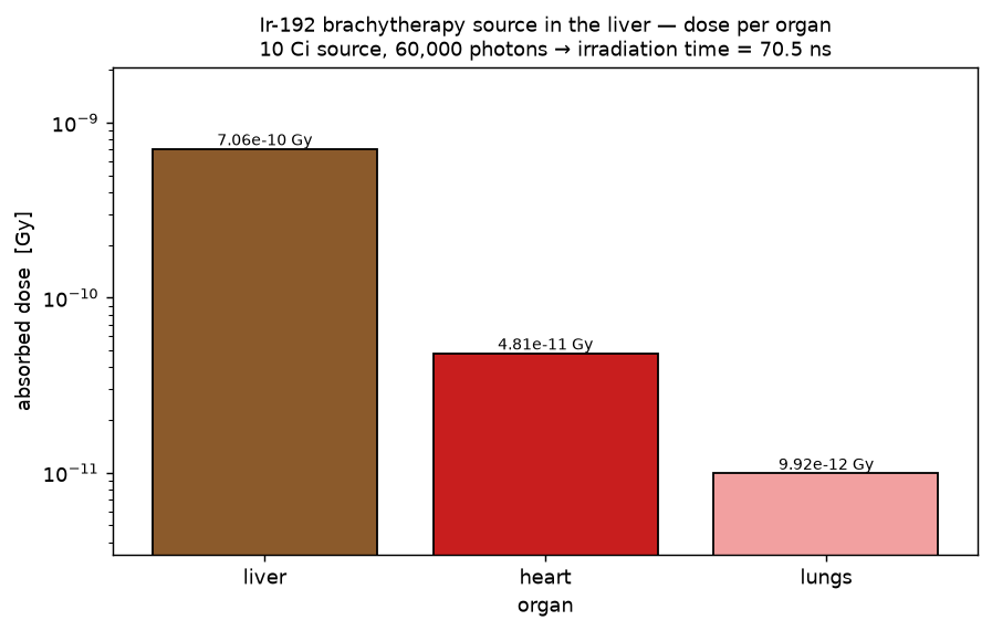
The liver, which hosts the source, absorbs by far the largest dose; the heart just above it and the lungs at the top of the stack receive a much smaller scattered dose — the localisation that makes brachytherapy attractive. The title reports the Ir-192 irradiation time that the simulated photon count represents (see Irradiation time above).
Plotting with the GEMC Analyzer
Run GEMC with 200 events first. The default YAML file writes the analyzer CSV streams.
gemc cad.yaml -n=200
Plot the total energy deposited per hit:
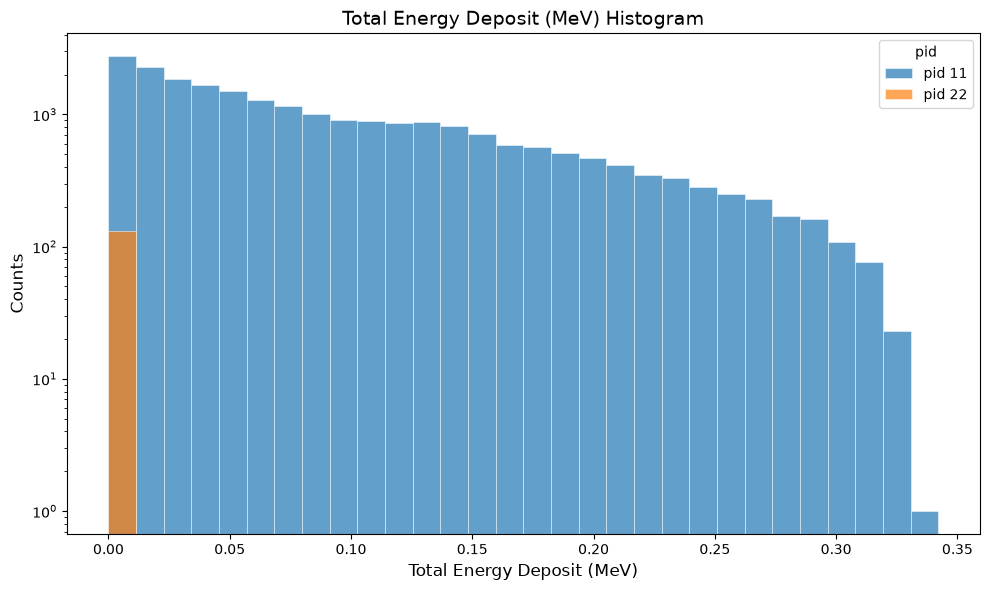
gemc-analyzer organs_t0_digitized.csv totEdep --kind csv